

\[ \begin{bmatrix} a & b & c \\ d & e & f \\ g & h & 1 \end{bmatrix} \begin{bmatrix} x \\ y \\ 1 \end{bmatrix} = \begin{bmatrix} wx' \\ wy' \\ w \end{bmatrix} \]
\[ \begin{cases} ax + by + c = wx' \\ dx + ey + f = wy' \\ gx + hy + 1 = w \end{cases} \implies \begin{cases} ax + by + c = (gx + hy + 1)x' \\ dx + ey + f = (gx + hy + 1)y' \end{cases} \implies \begin{cases} ax + by + c - gxx' - hyx' = x' \\ dx + ey + f - gxy' - hyy' = y' \end{cases} \]
\[ \implies \begin{bmatrix} x & y & 1 & 0 & 0 & 0 & -xx' & -yx' \\ 0 & 0 & 0 & x & y & 1 & -xy' & -yy' \end{bmatrix} \begin{bmatrix} a \\ b \\ c \\ d \\ e \\ f \\ g \\ h \end{bmatrix} = \begin{bmatrix} x' \\ y' \end{bmatrix} \]
Thus, given some n amount of correspondence points, we can stack these equations to form a 2n * 9 matrix A. For each correspondence point (x, y) -> (x', y'), we formulate two equations:
x'(h31x + h32y + h33) = h11x + h12y + h13
y'(h31x + h32y + h33) = h21x + h22y + h23
These equations are what is used to construct A.
Afterwards, we use SVD on A to solve for AH = b to construct H, which is our homography matrix.
For warping, we take our Homography matrix H, and inverse it to an adjusted cordiante plane and warped points. This essentially maps out points in the warped image to the original image that we are attaching the warp to.
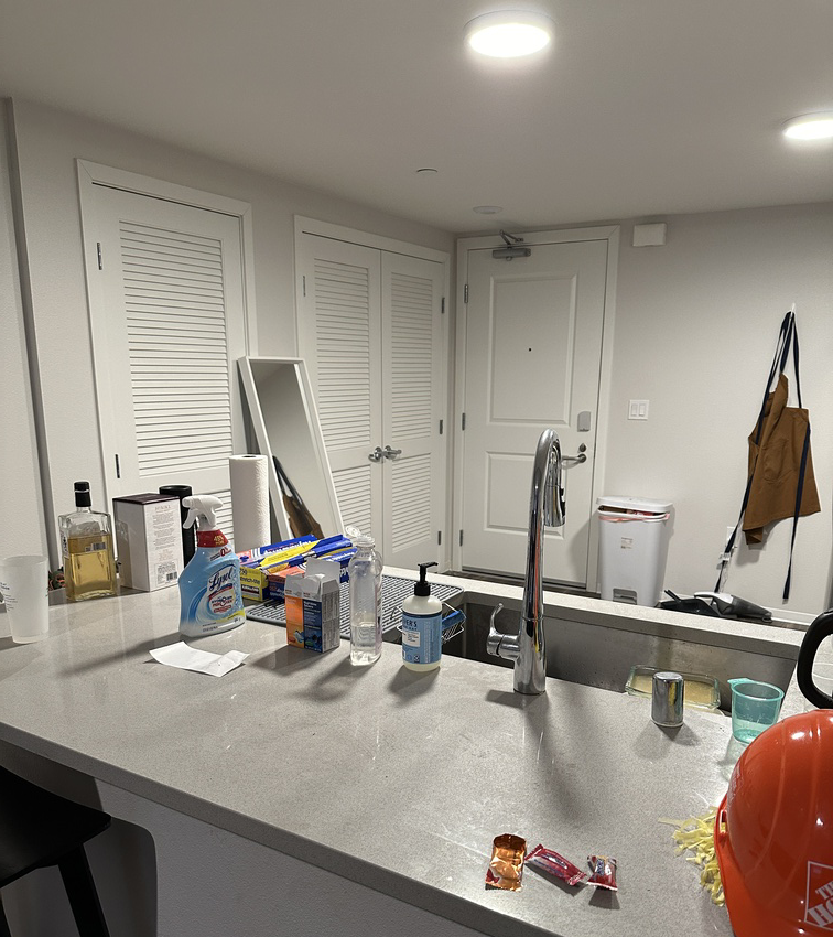
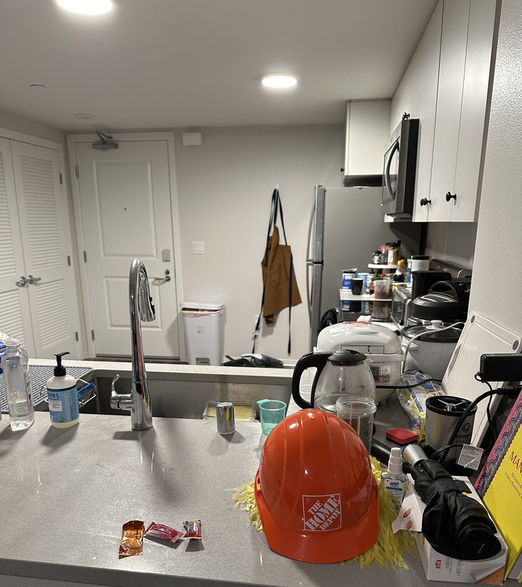
Below are the correspondence points for the 'Counter' Images that I used.
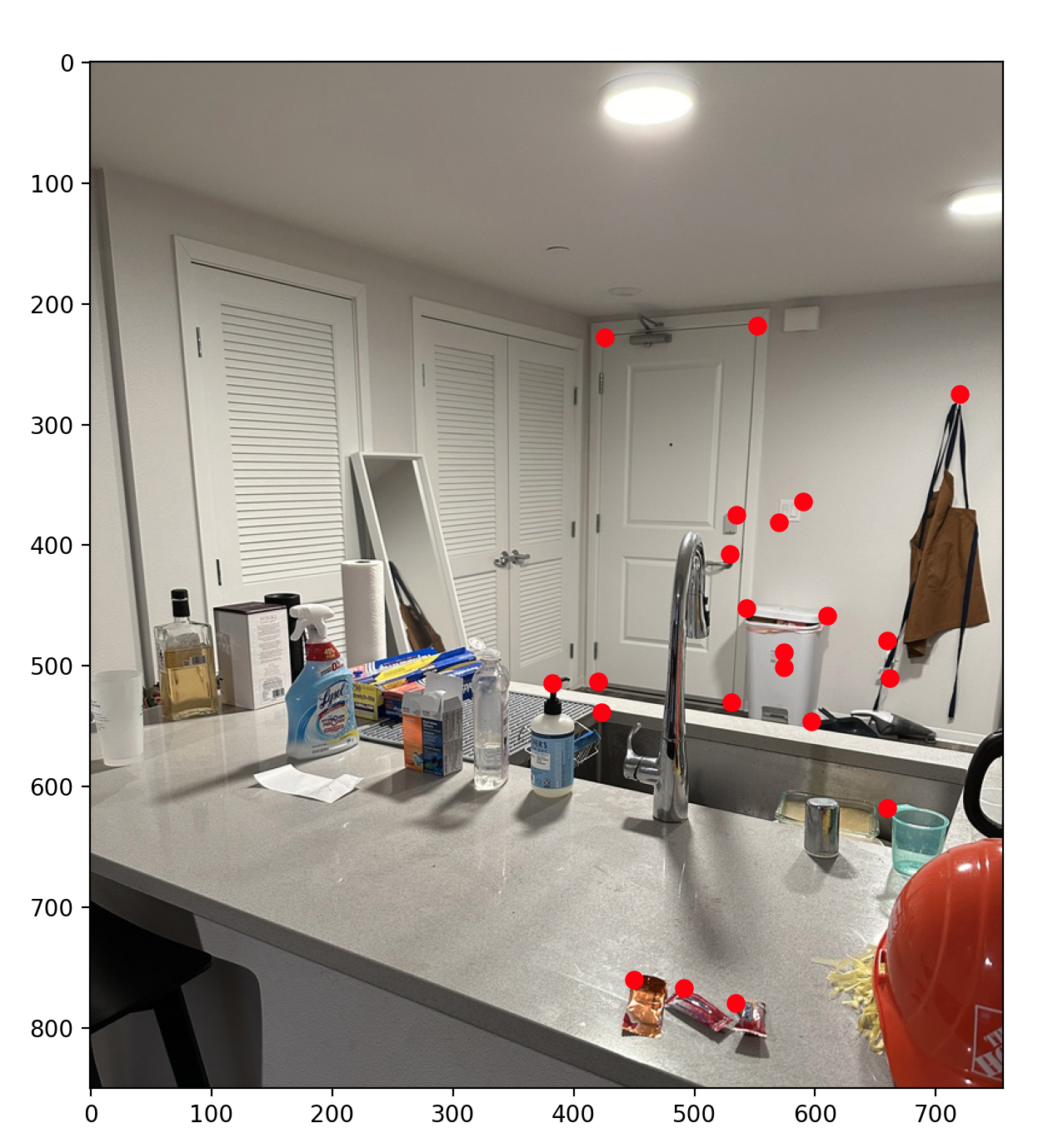
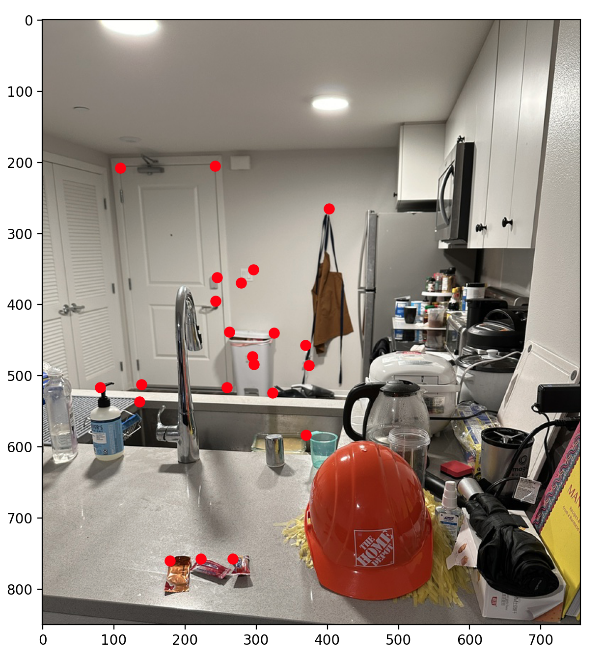
Afterwards, we can apply warp either Counter 1 to Counter 2, or vice versa. Shown below are both results!
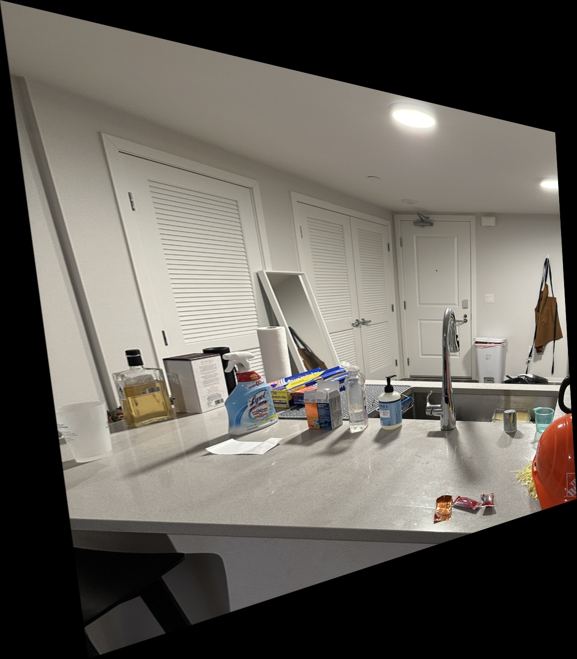
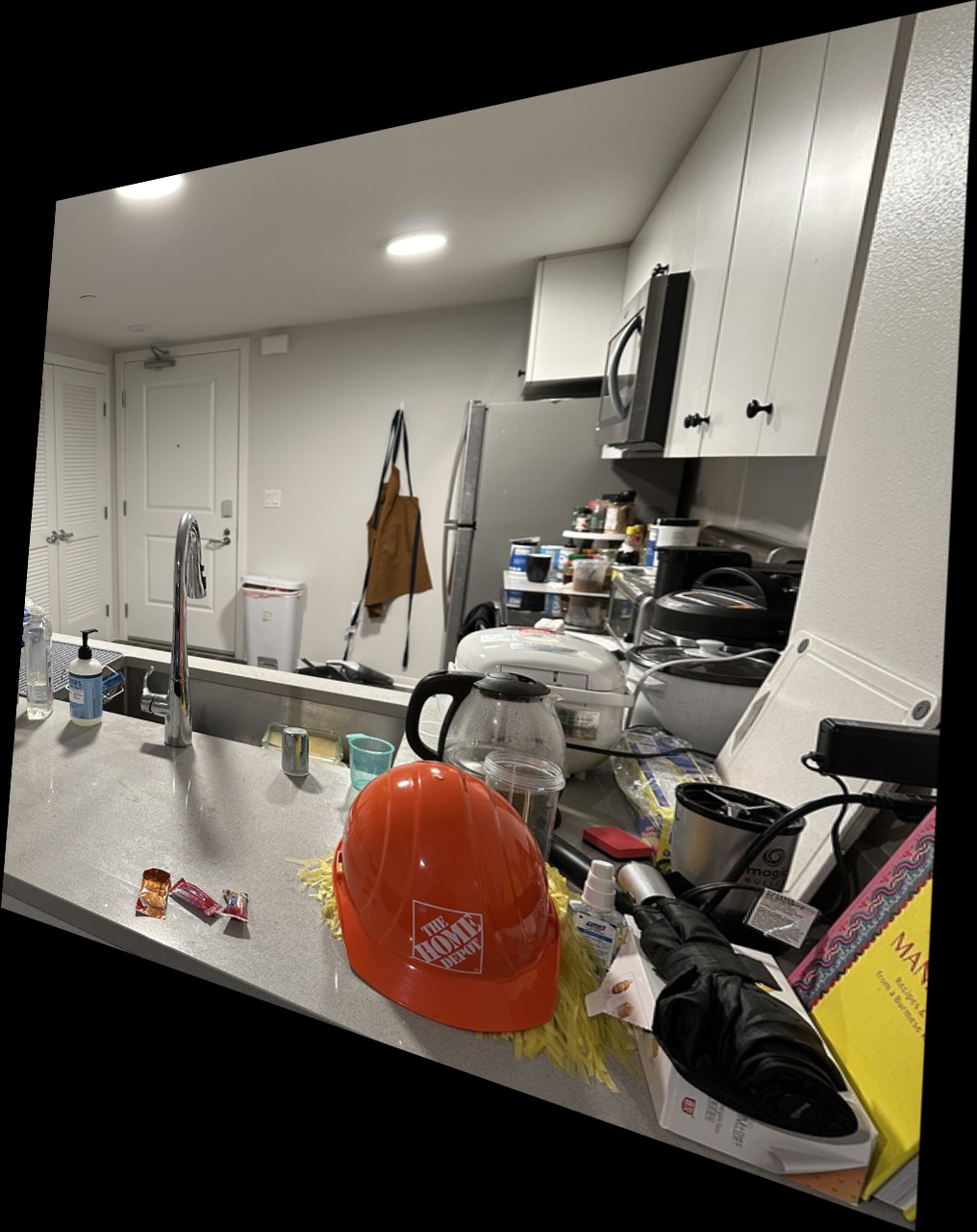
NOTE: Warping the same image to itself results in the same image! A good sanity check to ensure you warp function isn't doing something crazy...
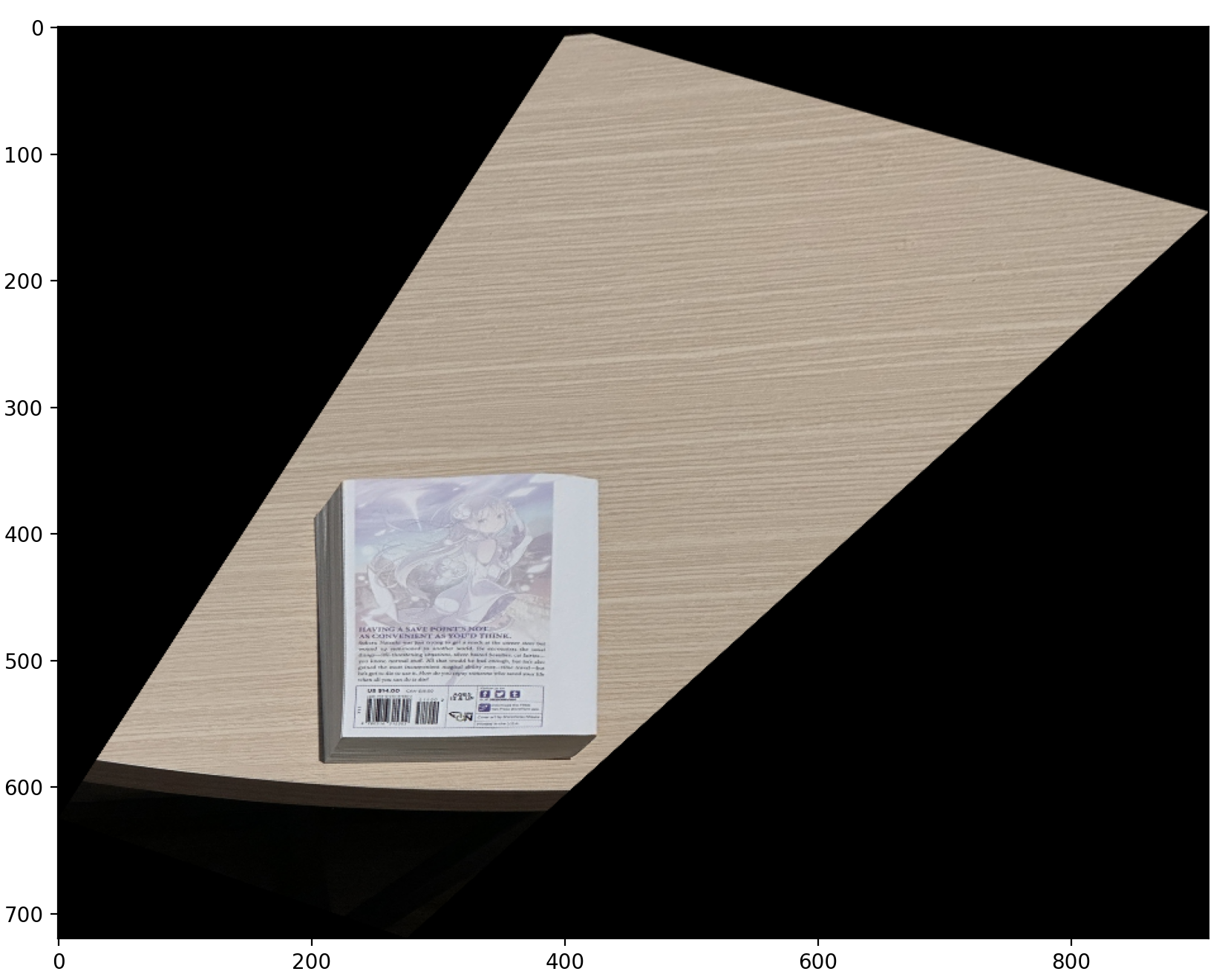
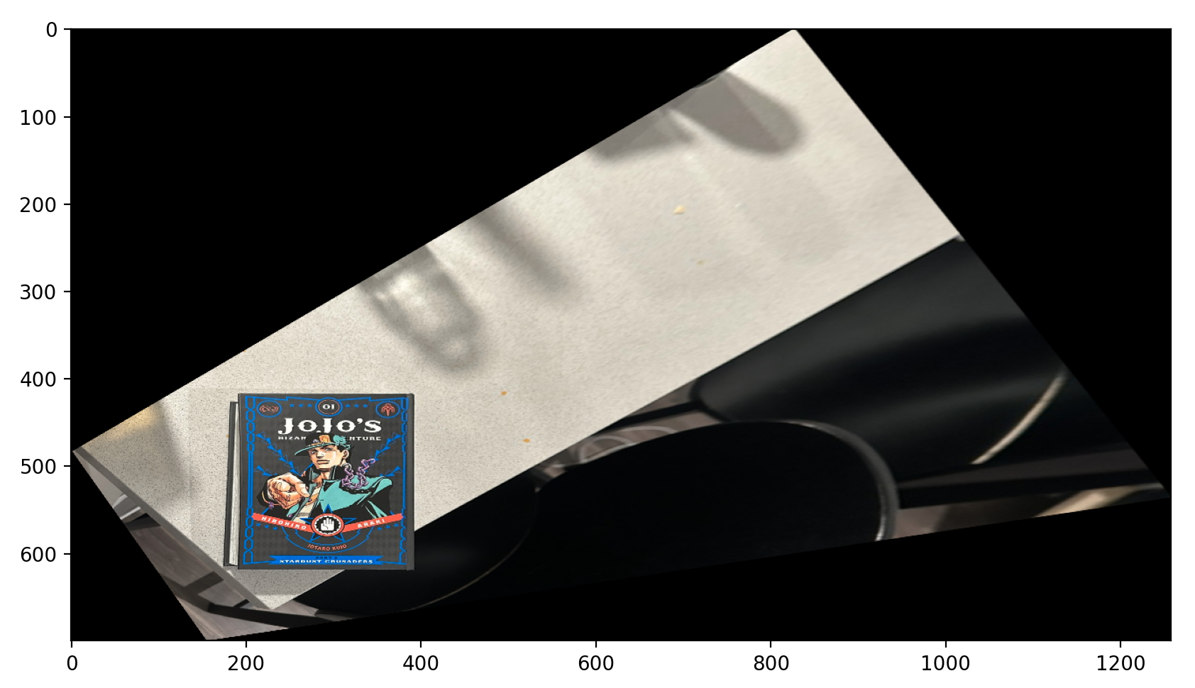
Given that we are able to warp our images, we can rectify specfic objects in an image! Essentially we take a irregular quadilateral and can turn it into a regular rectangle. This can be done by selecting the correspondence points soley around the corners around the area of desire and choosing the second set of points as the corners of the image.
Below are two examples of image rectification on some books that I enjoyed reading!
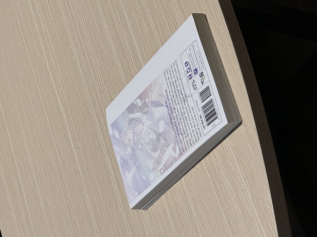
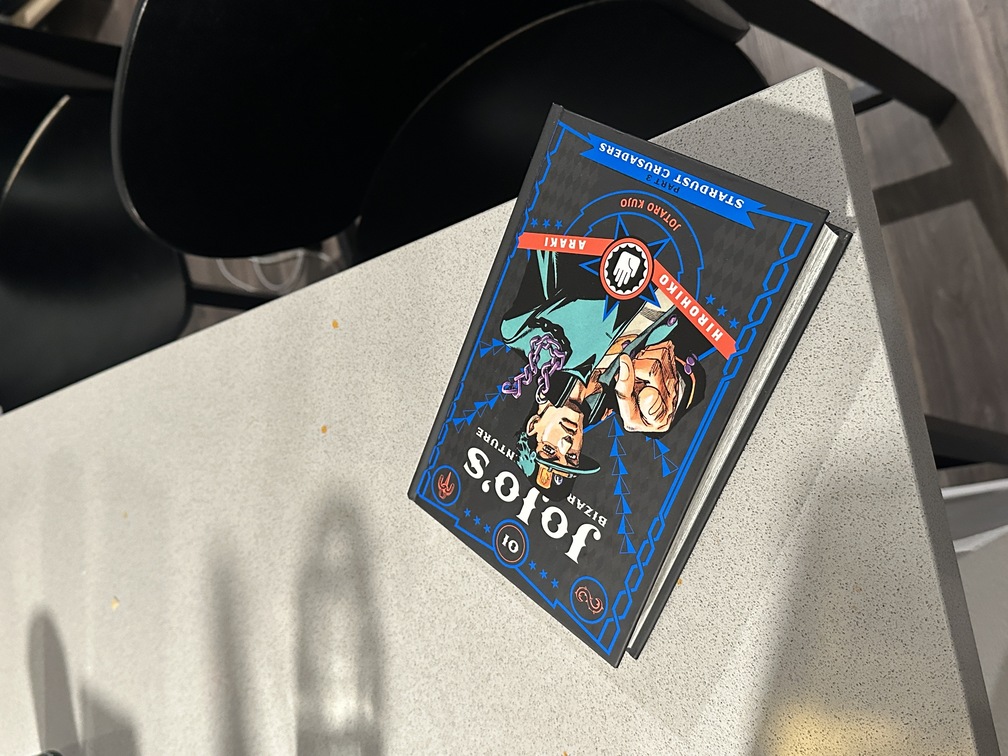
And the results...
Finally, using our warping function, we can construct a mosaic between warped and original images (even warped to warped images if you really want).
The process goes as follows... Compute Homography Matrix H between correspondence points from both images and choose either image (in our case, the first one, even both work). Given this image and H, we then apply our warping. During our warping process, I also specifically constructed output based on the warped image to help in creating the width and height of the final mosaic, as well as accomodating for any translatons. Afterwards, we place the warped image on the left and the unaltered second image on the right. Finally, to ensure clean results, we apply some blending techniques from Project 2. The only difference is, we have to accomodate for an irregular mask here. We can construct one by creating binary masks of both images on where there are pixels located and computing the distance transform on each of these masks to create weights for each image. The lowest frequency component is then blended using weights computed from distance transfoms. For the higher frequency, we use a binary to select between the two images based on which is closer at each pixel. Here we showcase two standard examples, one simple example, and one more extreme example of mosiacs created from the pictures.


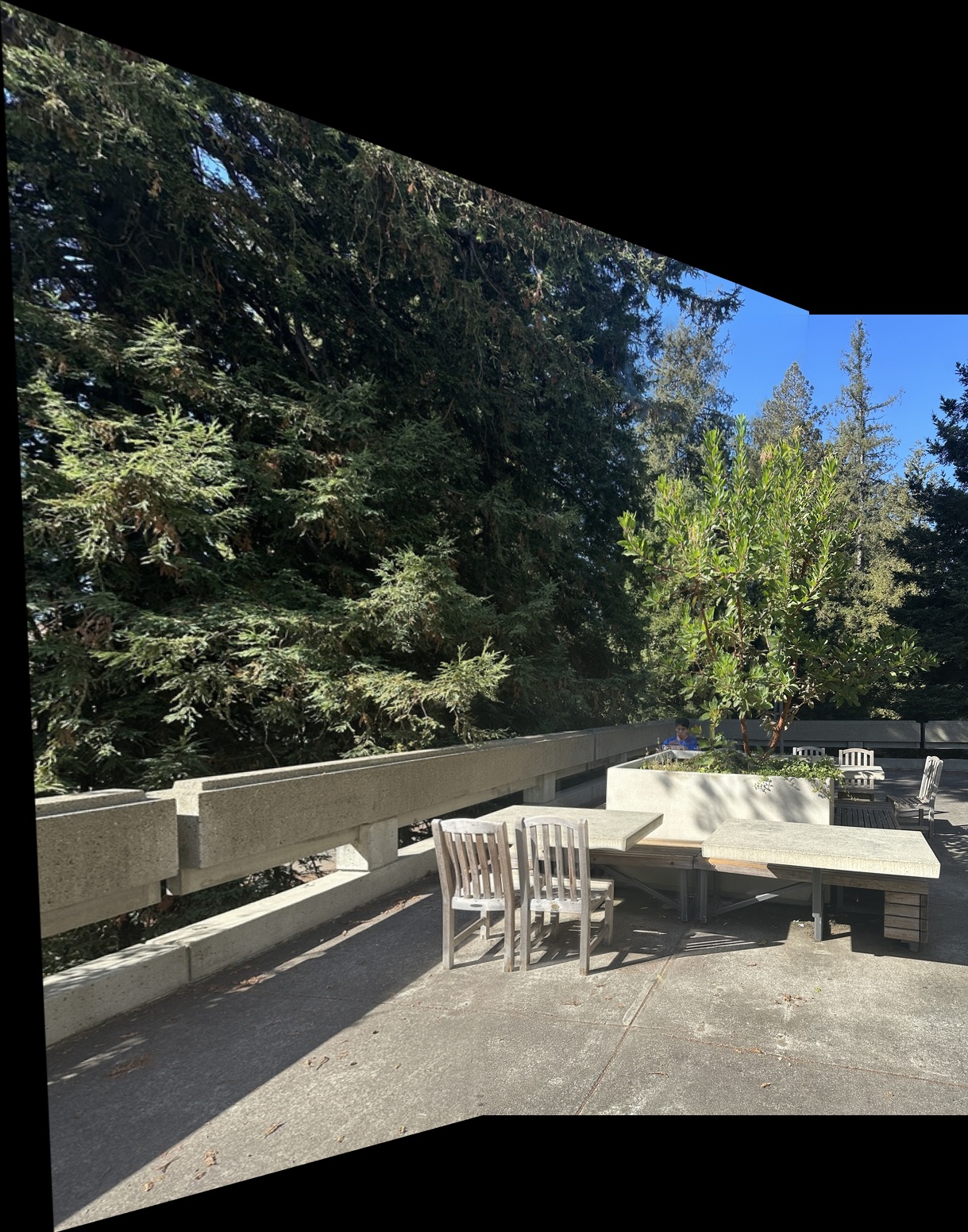


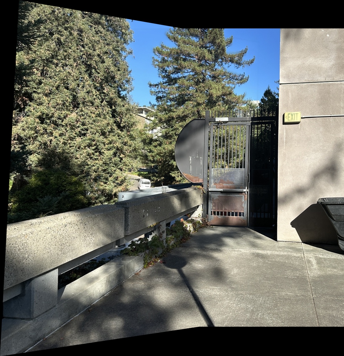


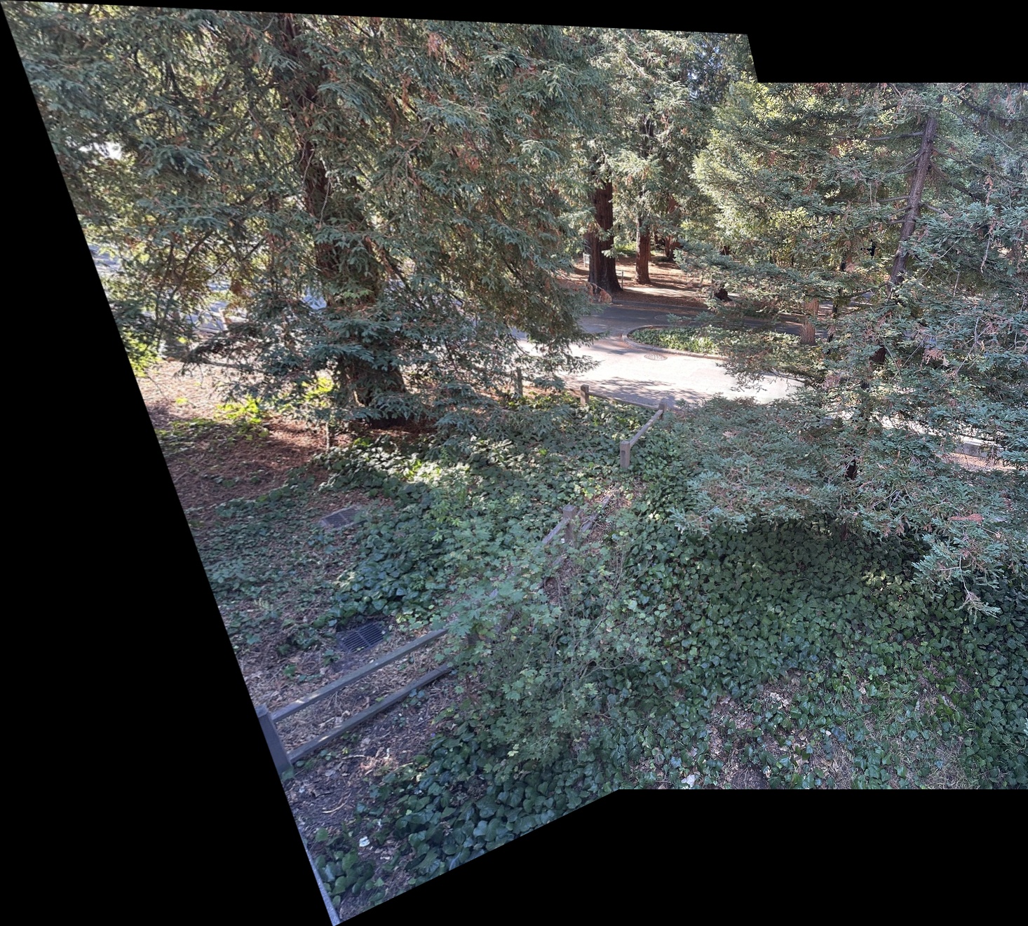
Alright, now we start the next portion of the project!. Previously, we had to select points in the images that we could use as correspondence points manually. This task was a pretty big hassle and DID NOT build any character =[. So, for this section, we'll be automating this process!
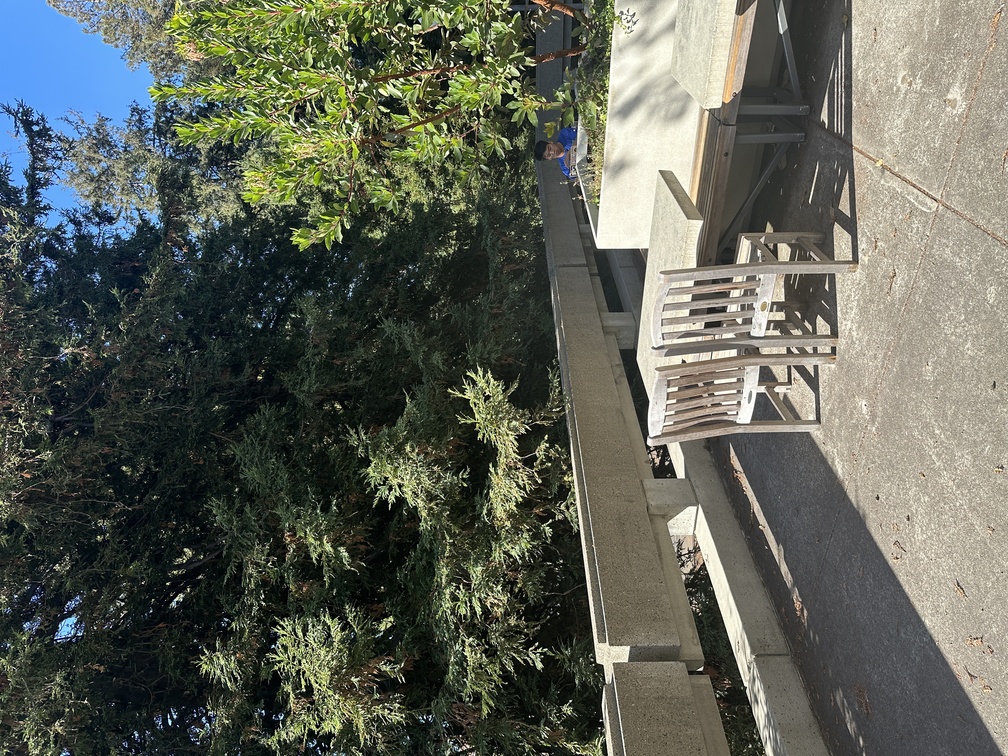
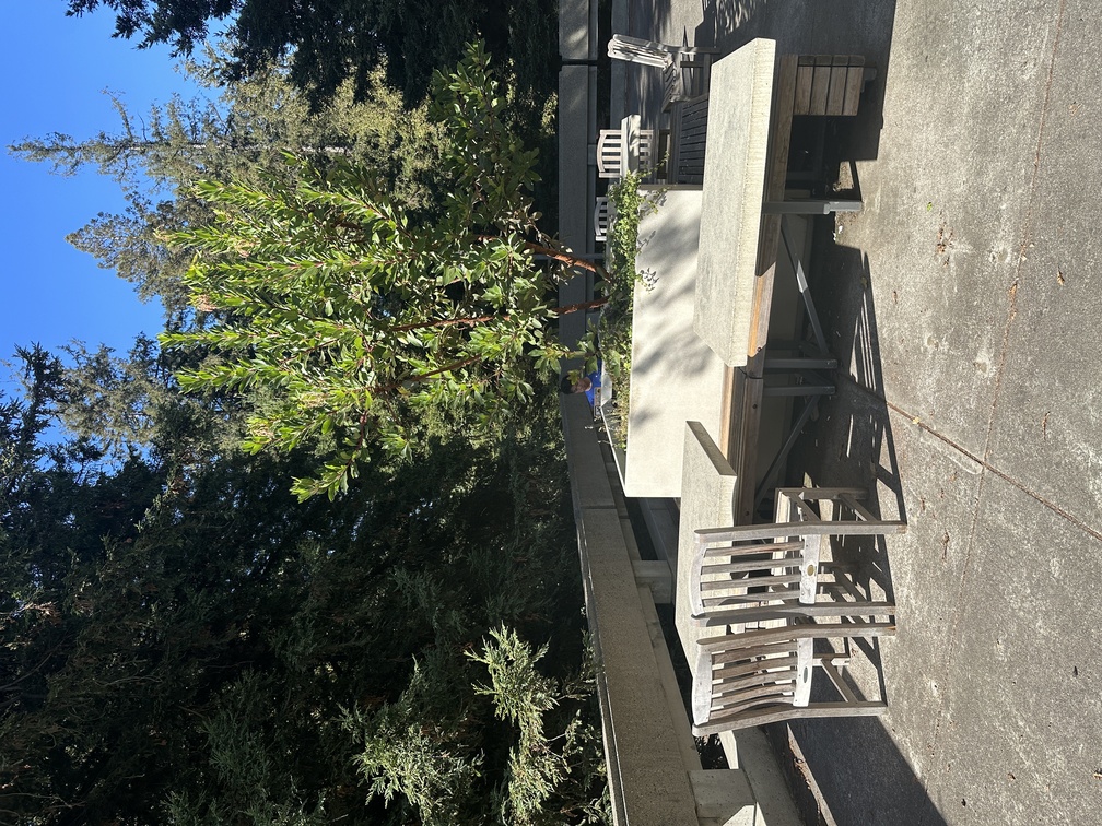
Before we start, we utilized another set of images for testing.
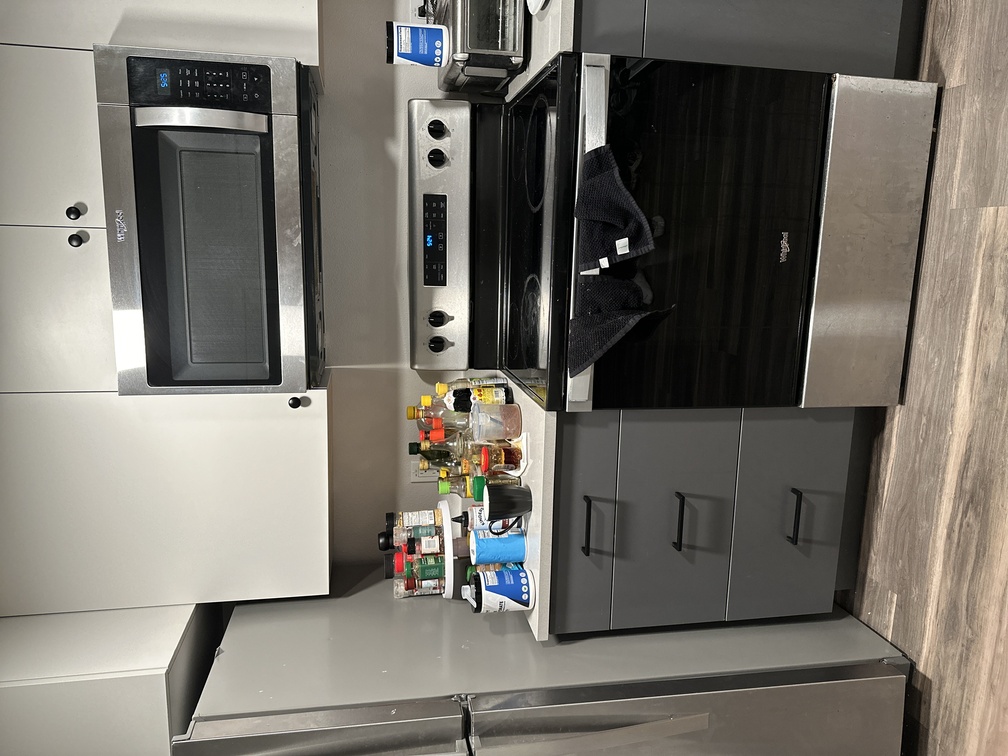
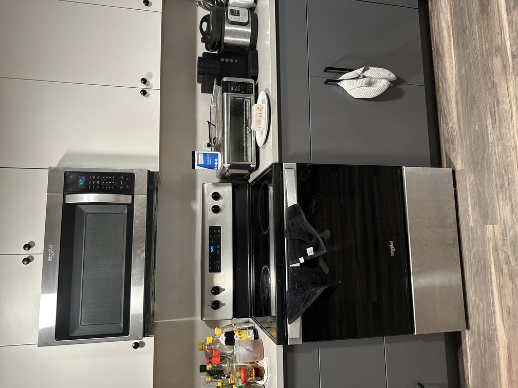
How we'll be accomplishing this is by the following: (1) Detecting corners from an image. (2) Extracting feature descriptiors from the images given the corners. (3) Matching these descriptors to the images. (4) Using Ransac to compute a homography. (5) Using what we built in Part 4a to warp the images together.
Below is the naive Harris Detection Code that was provided as you can see on the left. On the right, we implemented AMNS to select the points. I believe my AMNS looks better than other people simply due to the high amount of points that are available in the image, and how well-defined the corners are. For reference, there are 500 points on the right that are outputted.
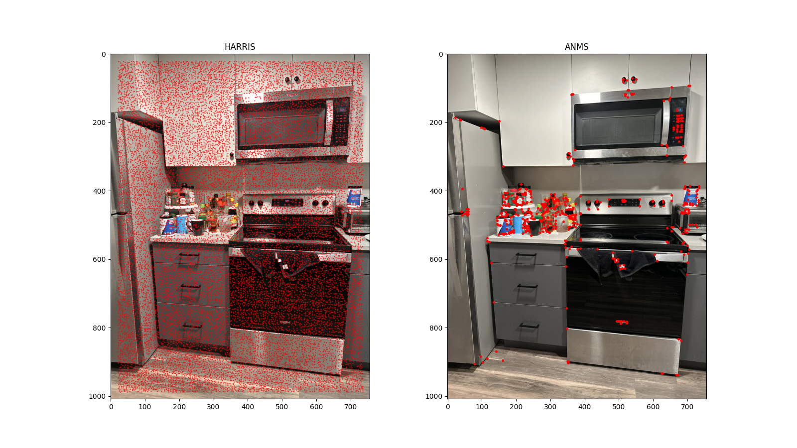
To accomplish this, we implement the Adaptive Non-Maximal Suppression (ANMS) process. First, we sort the corner points based on their Harris response strength. For each corner point xi, we find all points that have a strength greater than 0.9 times the response strength of xi. This helps us identify stronger points in the vicinity. Next, we calculate the minimum distance from xi to these stronger points, which we designate as the point's "suppression radius." Finally, we select the top 500 points with the largest suppression radii.
From the ANMS points, we iterate through each one and extract a square patch of size (40x40). To ensure noise doesn't play an effect, we apply a Gaus Blur.
For each of the patches, we can resize it to a 8x8 descriptor. Finally we vectorize and normalize it.
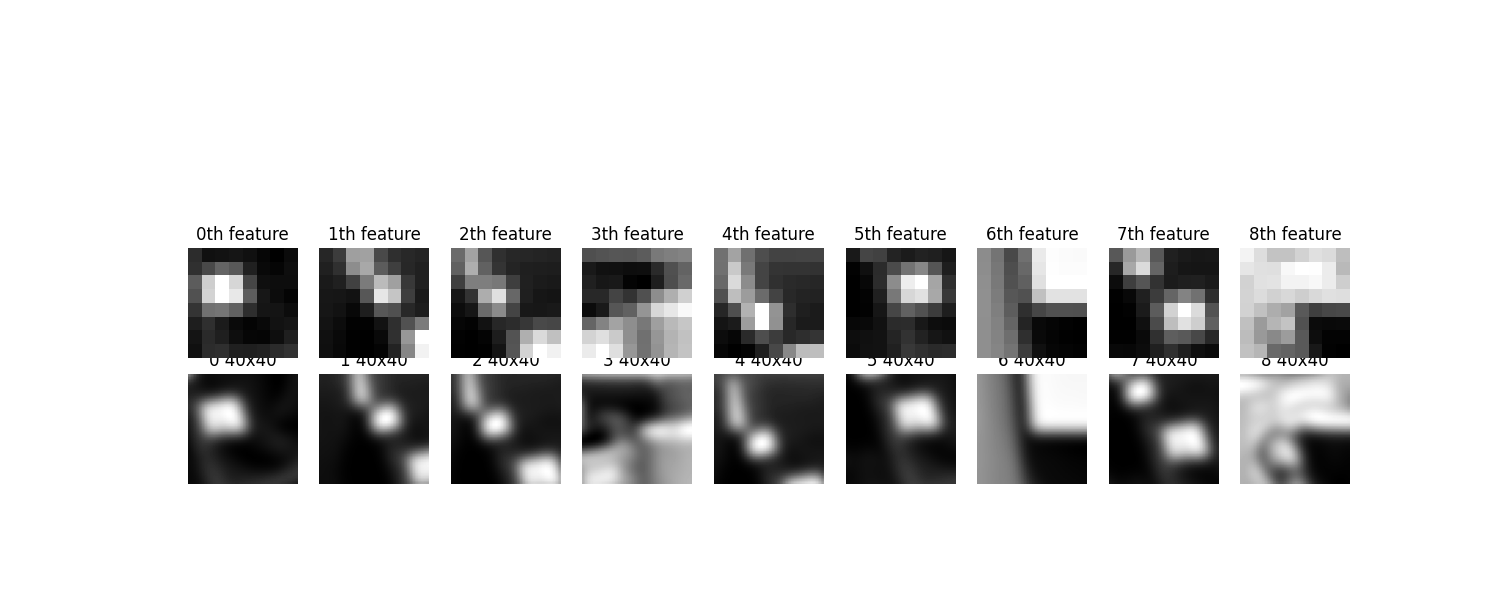
We do this because even though we have these points, we want to gain some 'feature' from them for matching, which is the next section!
Afterwards, we can now use these descriptors to start matching features with one another, which we can use to create correspondences. This means we'll be repeating the above process twice.
For each image, we iterate through each feature of the image and match it to whatever is the best matching feature of the other image. We utilize KDTrees for this for efficient querying.
Afterwards, we ensure that a match in one direction is also the best match in the other direction. If not, then we do not include it.
To ensure highest quality, we also utilzed Lowe's ratio test, which we used to compared the closest and second-closest feature matches. If it is the case that these distances are too close to one another, then we consider teh match unreliable.
Below are the results of doing the outlined steps.
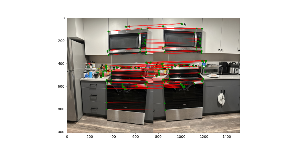
Some matches can be misleading, hence why we utilize RANSAC to further reduce the number of outliers, since outliers can greatly change the output.
We randomly select 4 pairs of points, then we compute the homography matrix given these points. During this process, we construct a list of inliners frmo this homography matrix.
For each point in an image, we determine the other images warped position by using the homography. Then, using the literal position of the point of the other image and determine if the distance between the estimated point from the homography matrix and the original point vs the actual point from the other image is less than some error (this is to ensure robustness). If it is the case, then we add it to the list of inliners.
After some predetermined amount of iterations (500 in my case), we use the homography that constructed the most amount of inliners.
Below are some of my results:
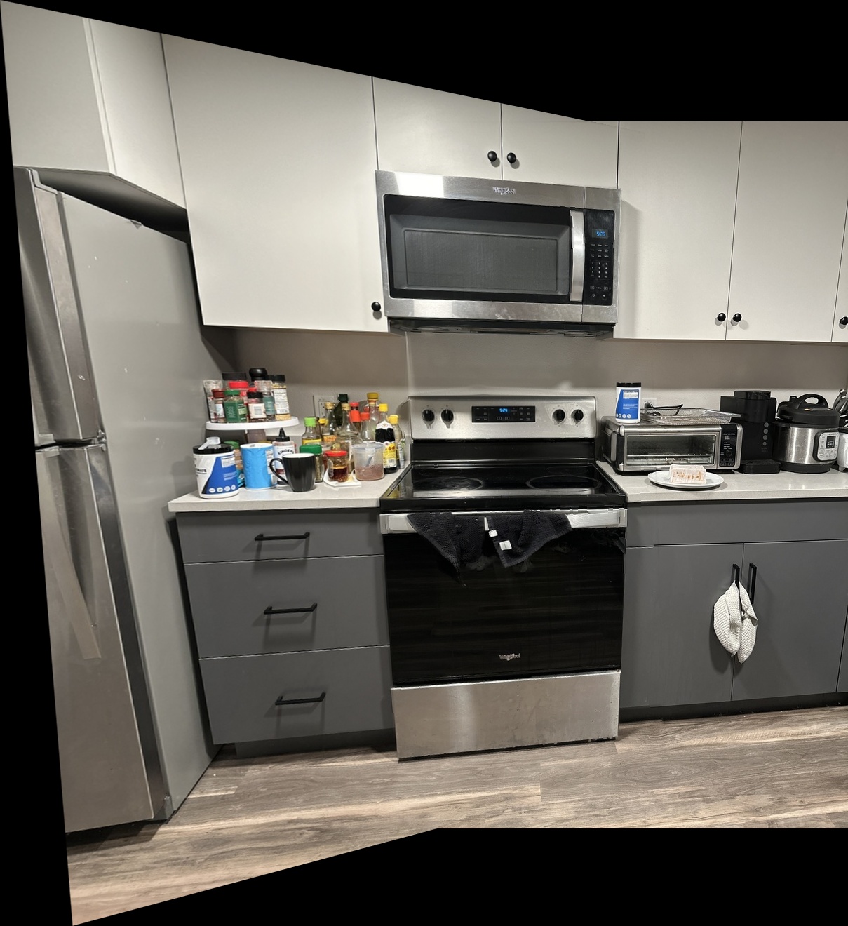
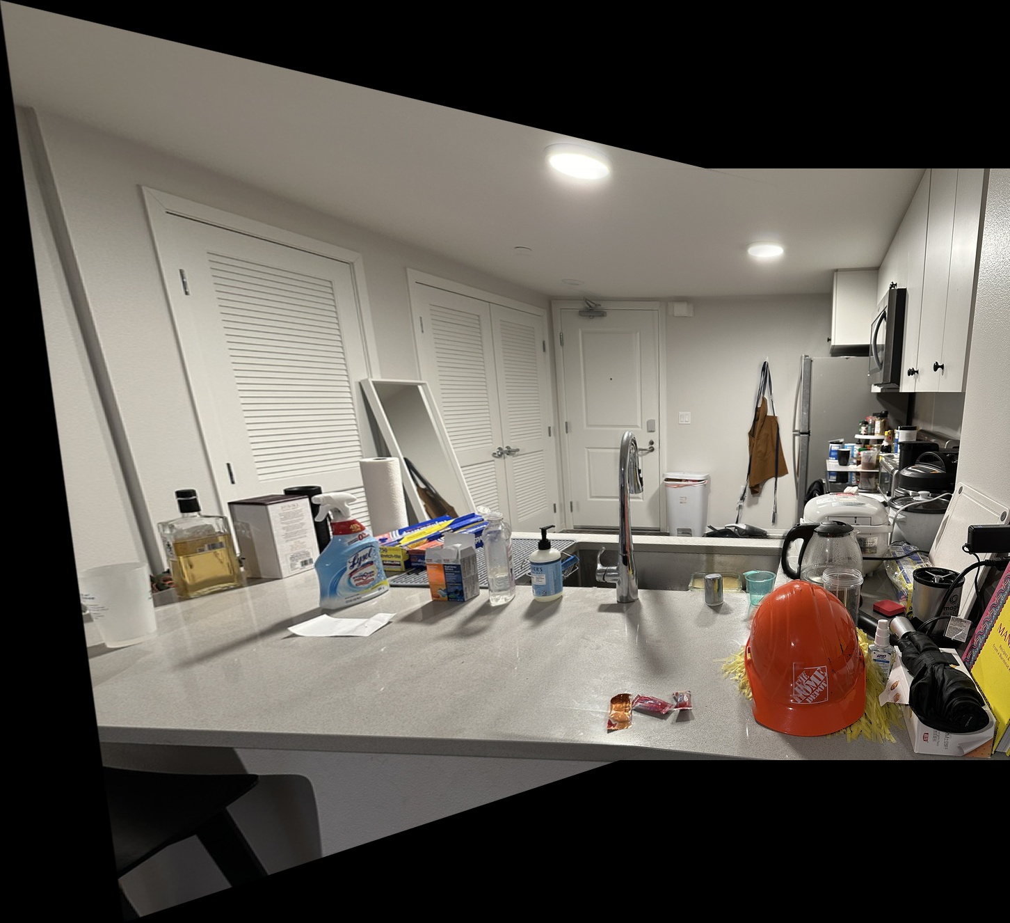
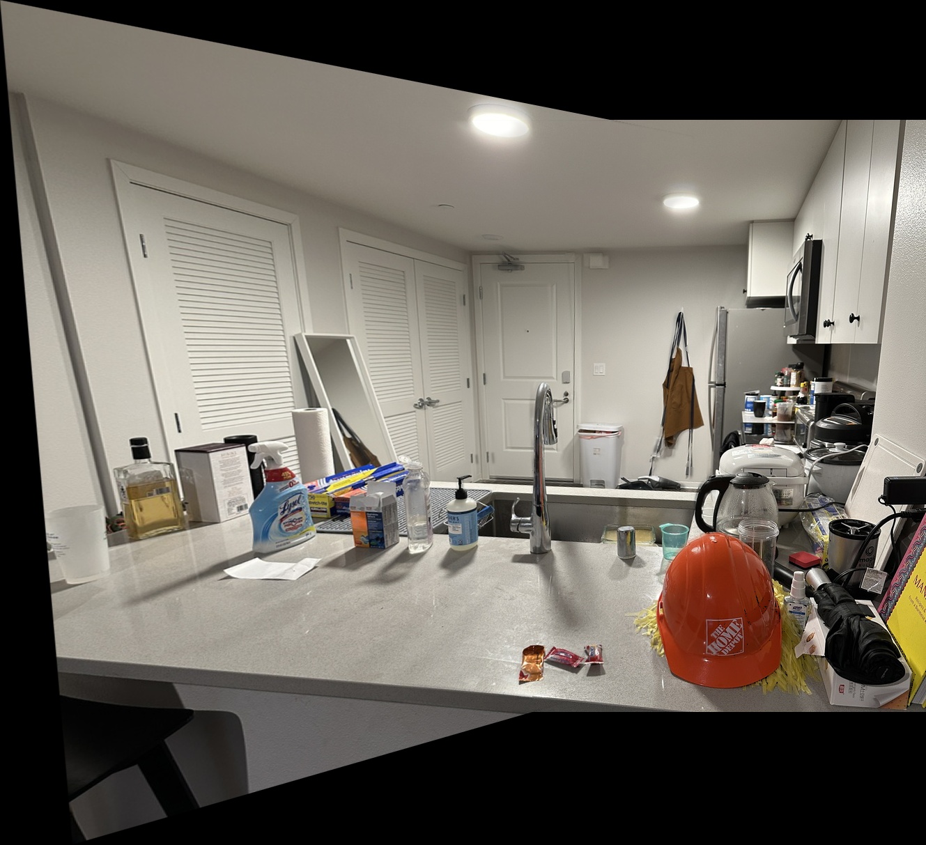

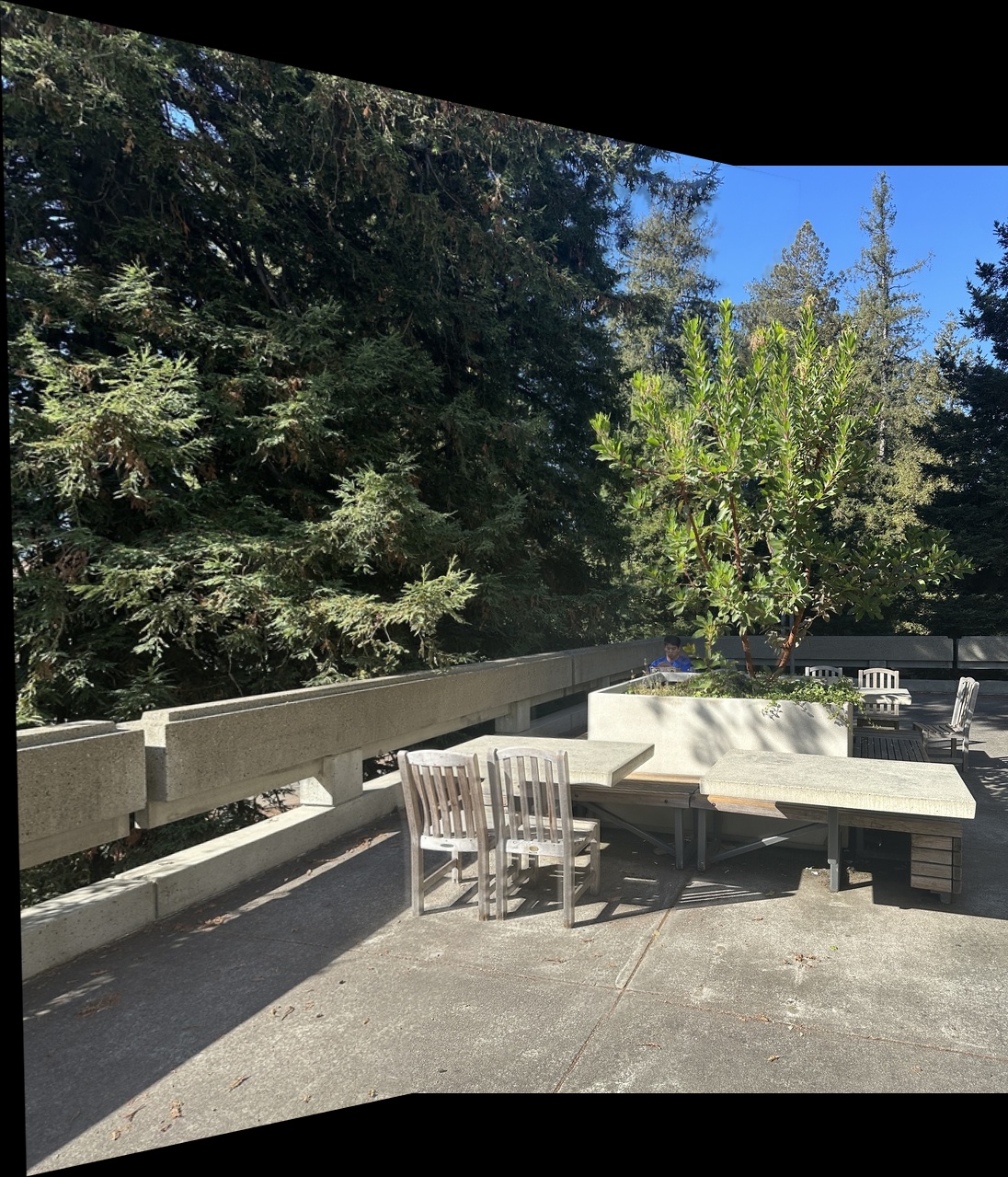
Give or take the automated selection of points does a reasonably good job compared to when I was manually clicking. If you include the actual effort that went into clicking all those points, I'd say these results are very successful!
Learning how to filter out harris corner detection and make the outputs more robust is DEFINIETLY something that I'll be using for my future work. In hindsight, probably the most useful content that I have seen (at least from what I can tell).